Demystifying Neural Nets with The Shapley Value
Unboxing The Black Box with The Shapley Value and Game Theory
Explainability of deep learning is quickly getting its momentum despite its’ short history. Explainable AI derived from the rising demand for fairness and justice of neural networks’ decisions and to avoid coded bias. So-called black box AI could make assumptions and predictions of one entity based on a bias that resonates with the real world. Many techniques sprouted to mitigate such deleterious impact on people, especially on social minorities. The core function of these techniques is to explain the neural networks decision process and its behaviour. One of the most widely utilized tools to explain the model’s behaviour is called feature importance. However, this turns out not to be the most trustworthy and robust method to reflect the model’s true behaviour. Here is why:
Feature Importance
- First and foremost let’s understand how feature importance operates. Feature importance measures increase in the model prediction error after permuting feature’s values. What this would mean is that the “importance” of a feature is defined by the model’s reliance on that feature. If the model error increases after shuffling the values of the feature, it implies that the feature played a big role in the prediction. Reversely, if the model error remains stagnant after shuffling, that feature would probably didn’t do much on the model’s decision.
- However, feature importance only operates correctly on linear models. This is due to the nature of feature importance that it adds up both the main feature effect and the interaction effects with other features. Thus, any feature with a negative result is added up with a positive result. It’s like squashing the result into one big piece. The result is it that it doesn’t really reflect the individual negative and positive effects of the feature.
- Additionally, adding correlated features makes the interpretation of the output more complex. Let’s say there was a single important feature ‘treadmill’ for weight loss. Now I added ‘stairmill’, which is also effective for weight loss. Let’s also assume that the stairmill and treadmill are highly correlated. Now all of those two features are pulled down to the mediocre level in the feature importance plot instead of remaining in the top position. Such an outcome requires extra time and effort to interpret the result.
The Shaley value is great alternative to overcome such drawbacks. So what exactly is the Shapley value?
Shapley Value
The Shapley value stems from game theory. Game theory is a study of interactive decision-making among rational agents. In the instance of the game, logical players the decision-makers would make strategic decisions depending on the actions of other players to win the game or achieve their desired goals. The Shapley value becomes handy when assessing how much each participant contributed to the result of the game. The value is calculated by weight averaging the marginal contribution of all agents across all possible coalitions. In machine learning, the player or the agent corresponds to the feature and the importance of that feature is computed with the Shapley value. Below is the equation to get the Shapley value. Looking at descriptions written in human language underneath the formula would be helpful to interpret the formula.

Enough with all the mathematical symbols and let’s understand the value with a real-world example. There are two players and four different games. In the first game, both players did not play the game. In the second game, only player 1 played. For the third game, only player 2 played. In the last game, all players participated. The prediction column represents the predicted value for each case. Bullet points below explain how you can calculate the Shapley value.


Unlike feature importance, which would add a negative effect with positive interaction effects and main feature effects all at once, Shapley values takes into account the decrease in performance. Furthermore, it is more robust in generating the result. The upsides of the Shapley value doesn’t stop here. It works not only with linear models but also with neural networks! You can interpret any machine learning model with this value.
You can easily implement this value using SHAP(Shapley Additive exPlanations) library in python. The downside of the SHAP is that it is computationally expensive and slow. Additionally, one needs to be aware that the Shapley value should never be interpreted as a causal relationship. Just because a certain feature was helpful for the prediction does not always imply causation.
You may face some errors due to version incompatibility issues with Tensorflow. I’ll explain how to fix those here and run a simple experiment. The contents of the experiment cover image classification of American style make-up vs. Korean style make-up and which features contributed to the model’s prediction.
This is not an extensive experiment but to quickly check how SHAP could be applied in neural networks. In this experiment, I used a CNN model trained on a small dataset. Thus, the result may significantly improve by enlarging the dataset size. You can access the detailed code and dataset via this link.
Here are very useful tips to solve errors while implementing SHAP.
Resource exhausted: OOM when allocating tensor with shape[ , , ,]
When you run into this problem try these two steps:
- Reduced batch size to 16 (could be larger or smaller but to the point that it wouldn’t show the corresponding error)
- Reduce input dimension to 100 (could be larger or smaller but to the point that it wouldn’t show the corresponding error)
If you are using Tensorflow version > 2.4.0
Restart the runtime and include the following code at the very top of your code.
import tensorflow as tf
import tensorflow.compat.v1.keras.backend as K
tf.compat.v1.disable_eager_execution()
Experiment
I have two folders that consist of training sets and test sets. Each image in the folder is sorted into two classes: ‘american_makeup’ and ‘korean_makeup’.
base_dir = '/content/gdrive/MyDrive/research/images'
train_dir = os.path.join(base_dir, 'train')
test_dir = os.path.join(base_dir, 'test')class_name = os.listdir(train_dir)
class_name_test = os.listdir(test_dir)print(class_name)
#['american_makeup', 'korean_makeup'] print(class_name_test)
#['american_makeup', 'korean_makeup']
As of now, each class is written with a categorical variable. I need to encode them into integer variables. Here I used LabelEncoder to change class names to an integer. Once you are done with integer encoding, the next step is to perform one-hot encoding. The class name ‘american_makeup’ is now labeled as [1,0] and ‘korean_makeup’ is labeled as [0,1].
integer_encoded = LabelEncoder().fit_transform(class_name)
integer_encoded = integer_encoded.reshape(len(integer_encoded), 1)onehot_encoded = OneHotEncoder(sparse=False).fit_transform(integer_encoded)print(onehot_encoded)
#[[1. 0.]  [0. 1.]]integer_encoded_test = LabelEncoder().fit_transform(class_name_test)
integer_encoded_test = integer_encoded_test.reshape(len(integer_encoded_test), 1)onehot_encoded_test = OneHotEncoder(sparse=False).fit_transform(integer_encoded_test)print(onehot_encoded_test)
#[[1. 0.]  [0. 1.]]
Training dataset and test dataset are resized and reshaped and saved into new lists. Each of the corresponding labels is stored in train and test label lists.
train_image = []
train_label = []
test_image = []
test_label = []# for train dataset
for i in range(len(class_name)):
    path = os.path.join(train_dir, class_name[i])
    img_list = os.listdir(path)
    for j in img_list:
        img = os.path.join(path, j)
        img = cv2.imread(img, cv2.IMREAD_COLOR)
        img = cv2.cvtColor(img, cv2.COLOR_BGR2RGB)
        img = cv2.resize(img, (100, 100), interpolation =
              cv2.INTER_CUBIC)
        img = img.reshape((100, 100, 3))
        train_image.append(img)
        train_label.append(onehot_encoded[i])# for test dataset
for i in range(len(class_name_test)):
    path = os.path.join(train_dir, class_name_test[i])
    img_list = os.listdir(path)
    for j in img_list:
        img = os.path.join(path, j)
        img = cv2.imread(img, cv2.IMREAD_COLOR)
        img = cv2.cvtColor(img, cv2.COLOR_BGR2RGB)
        img = cv2.resize(img, (100, 100), interpolation =
              cv2.INTER_CUBIC)
        img = img.reshape((100, 100, 3))
        test_image.append(img)
        test_label.append(onehot_encoded[i])
There are few more steps that needs to be dome before applying SHAP. First, we need to normalize the data. Another important task is to actually know how your data is stored. American style make-up images were ordered first followed by Korean style make-up images in my dataset. In order to avoid any undesirable information leakage or learning I shuffled the whole data again.
# Normalize image dataX_train = shuffle(train_image.reshape(283, 100, 100, 3).astype("float32") / 255, random_state = seed)X_test = shuffle(test_image.reshape(20, 100, 100, 3).astype("float32") / 255, random_state = seed)
# Shuffle data or use library to randomly split your datatrain_label = shuffle(train_label, random_state = seed)
test_label = shuffle(test_label, random_state = seed)
Now you can finally design your model! The architecture of your model completely depends on how you would like to build your model as SHAP is model-agnostic!
def CNN():input_layer = keras.Input(shape=(100,100,3))x = keras.layers.Conv2D(150, (3,3), padding='same', activation = 'relu', kernel_initializer = keras.initializers.HeUniform(seed=seed))(input_layer)x = keras.layers.BatchNormalization()(x)x = keras.layers.MaxPooling2D((2, 2))(x)x = keras.layers.Conv2D(150, (3,3), padding='same', activation = 'relu', kernel_initializer = keras.initializers.HeUniform(seed=seed))(x)x = keras.layers.BatchNormalization()(x)x = keras.layers.MaxPooling2D((2, 2))(x)x = keras.layers.Conv2D(150, (3,3), padding='same', activation = 'relu', kernel_initializer = keras.initializers.HeUniform(seed=seed))(x)x = keras.layers.BatchNormalization()(x)x = keras.layers.MaxPooling2D((2, 2))(x)x = keras.layers.Conv2D(150, (3,3), padding='same', activation = 'relu', kernel_initializer = keras.initializers.HeUniform(seed=seed))(x)x = keras.layers.BatchNormalization()(x)x = keras.layers.MaxPooling2D((2, 2))(x)x = keras.layers.Flatten()(x)x = keras.layers.Dense(128, activation='relu', kernel_initializer = keras.initializers.HeUniform(seed=seed))(x)x = keras.layers.Dropout(0.5)(x)output_layer = keras.layers.Dense(2, activation='sigmoid')(x)model = keras.Model(inputs=input_layer, outputs=output_layer, name = 'CNN')model.compile(loss='binary_crossentropy', optimizer= keras.optimizers.SGD(learning_rate=0.001), metrics=['acc', 'AUC'])return model
After training the model, it was tested on ten American celebrity images and ten Korean celebrity pictures. Let’s see one of the example from the result.
idx = 6
input_val = X_test[idx:idx+1]
output_val = model.predict(input_val)
real = test_label[idx:idx+1]print("Prediction : ", np.argmax(output_val))
print("Ground Truth : ", np.argmax(real))plt.imshow(input_val.reshape(100, 100, 3),interpolation='nearest')
plt.show()
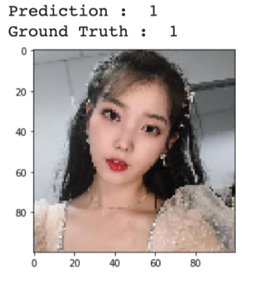
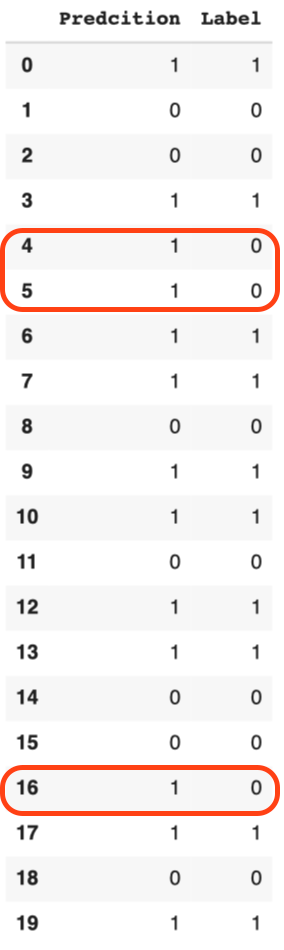
The model accurately classified the image! How about the rest? Out of twenty images, three were wrong.
I wonder what affected the model’s classification. Generally speaking, American make-up and Korean make-up have two very distinct styles. American make-up tends to highlight the shape of arched eyebrows, long fake eyelashes, and very smokey eye make-up. On the other hand, Korean make-up tends to desire very natural eyebrows, light shadows, clear make-up, and red-orangish lips. I am going to see if my guess is what really contributed to the model’s prediction.
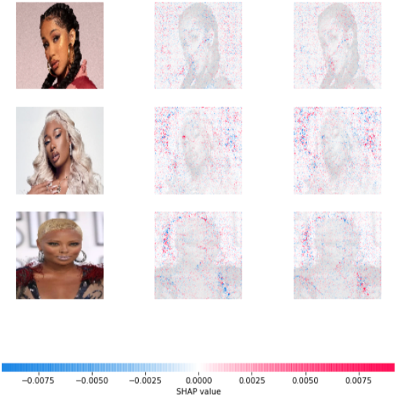
These are images of the American make-up style. Negative SHAP values refer to the negative impact and positive SHAP value refers to a positive impact on models decisions. The picture on the left is the groud-truth image. The one in the middle is label 0, which is American make-up style and the one on the far right is label 1, which is Korean style make-up.
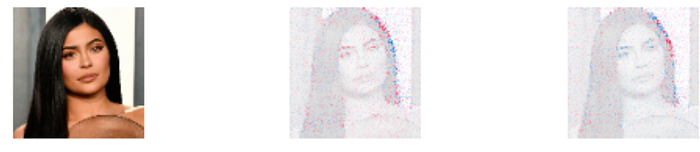


Surprisingly, red dots are concentrated around eyes and eyebrows for the middle image, which is label 0 (American make-up). Blue dots around eyes and eyebrows on Korean-style images suggest that those parts are telling that it is not Korean make-up images. Now let’s see the opposite result.


Korean style make-up is a lot less distinct compared to American make-up images. Nevertheless, we can guess that when the model classified images as Korean make-up it was largely due to the overall skin or structure of the face as red dots are spread across all faces.
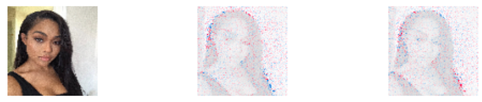
How about misclassified cases?
Here we can see that both labels 0 and 1 have red and blue points everywhere across the image. One interesting point is that all of the mislabeled cases are not white. Such results can provide very important clues where to fix and work on your model. In real-life settings, such biased outcomes can bring disastrous consequences and discriminate against certain groups of people.
How useful is the SHAP? What a time to be alive :-)
